
HarvestGroup360
© 2026 HarvestGroup360 — a brand operated by AMII LTD.
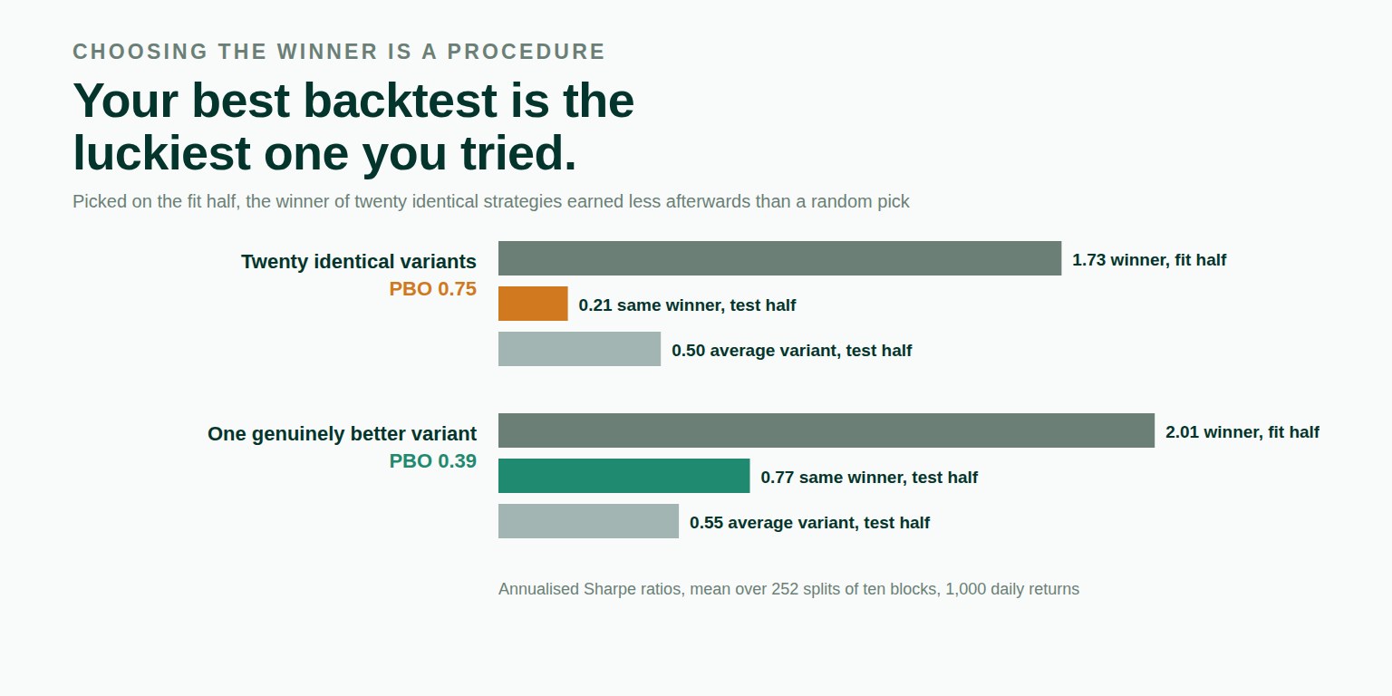
Twenty strategies with exactly the same edge. The one that looked best in-sample showed an annualised Sharpe ratio of 1.73 and went on to 0.21 out of sample — less than a strategy picked blindly. Choosing the winner is a procedure, and procedures can be tested.
Every backtest ends the same way. A grid of settings is tried — lookbacks, thresholds, stop levels, rebalancing windows — and the one that looked best is kept. Its Sharpe ratio is the one that reaches the deck, the investor letter or the forum post.
That figure always looks good, because it is the best of many tries. Report the top one of twenty variants and you are reporting the maximum of twenty noisy estimates. Some of it is skill and some of it is luck, and nothing in the number says how much of each.
The usual correction is the deflated Sharpe ratio, which asks how good the winner would have looked by chance and adjusts its figure. This article is about a different question, one that needs no assumption about how returns are distributed: does the act of choosing the in-sample winner pick something that keeps working?
The method is combinatorially symmetric cross-validation, published by Bailey, Borwein, López de Prado and Zhu in 2017. Cut the history into an even number of equal blocks, kept in time order so that anything serial inside a block survives. With ten blocks there are 252 ways to choose five of them as the in-sample half and leave the other five as the out-of-sample half. For each of those splits, find the variant that did best in-sample and record where it ranked out of sample.
If the winner lands at or below the out-of-sample median, that split counts against the procedure. The share of splits where that happens is the probability of backtest overfitting. A low value means the selection process can tell a better variant from a lucky one. A high value means it cannot.
We built the worst case deliberately. Twenty variants, a thousand daily returns each, every one drawn with the same true edge — an annualised Sharpe ratio of about 0.32. None of them is better than any other; every difference between them is noise. Ten blocks, 252 splits:
| Annualised Sharpe ratio | |
|---|---|
| Winner, in-sample | 1.7260 |
| Same winner, out of sample | 0.2128 |
| Average variant, out of sample | 0.4979 |
| Probability of backtest overfitting | 0.7540 |
| Degradation slope, out-of-sample on in-sample | −0.5604 |
gauss(0.0002, 0.01), 1,000 observations each, seeded. Annualised at 252 periods a year.On the whole history, the best of the twenty shows an annualised Sharpe ratio of 1.26 — for strategies whose true value is about 0.32. That is the number a single backtest of the winning setting would have reported.
We expected the probability to sit near one half on pure noise, and the first draft of the module's documentation said so. The worked example came back at 0.75, so we found out why before releasing it.
The reason is structural. The in-sample half and the out-of-sample half of every split are complements: together they are the whole sample. For any one variant, a stronger in-sample half means a weaker out-of-sample half for a given whole-sample result. On noise, choosing whichever variant had the best in-sample half systematically chooses one that is about to look worse. The sentence was corrected before release, and the changelog records that it was.
That check exists because of the fund fees release a day earlier, whose first documentation explained a correct number with the wrong mechanism and was corrected in a patch. Every figure and every stated mechanism is now re-run against the library after the text is written.
Now replace one of the twenty with a variant that has a genuine edge. Same method, same noise, same splits:
| Twenty identical | One genuinely better | |
|---|---|---|
| Winner, in-sample | 1.7260 | 2.0117 |
| Same winner, out of sample | 0.2128 | 0.7707 |
| Average variant, out of sample | 0.4979 | 0.5530 |
| Probability of backtest overfitting | 0.7540 | 0.3889 |
The better variant is chosen in 130 of the 252 splits. When the search contains something worth finding, the procedure finds it often enough, and the winner's out-of-sample figure sits above the average instead of below it.
That is the point of the measurement. It cannot say whether a strategy is good. It says whether the process that picked it can tell.
Both are required. The number of blocks decides how many splits exist and how long each half is; the metric — mean return or Sharpe ratio, with degrees of freedom stated — decides what “best” means. Either one changes the answer, so neither is chosen for you.
If the observations do not divide evenly into the blocks, the calculation stops and names the remainder. Dropping it silently would change the sample the answer describes.
Ties in-sample go to the first name in sorted order, and the out-of-sample rank counts only variants strictly below the winner. Both rules push a tie towards overfitting, never away from it.
from mdnorm import cscv

rep = cscv(variants, blocks=10, metric="sharpe", ddof=1)

rep.pbo                   # 0.7540
rep.mean_is_best          # how good the winner looked
rep.mean_oos_of_is_best   # what it went on to do
rep.mean_oos_all          # what an average variant did
rep.degradation_slope     # -0.5604
rep.chosen                # how often each variant won
$ mdnorm selection variants.csv --blocks 10 --metric sharpe \
--ddof 1 --annualise 252The last stretch of this series has been about numbers that depend on a choice nobody wrote down. Where the sample starts is a trial. Every cleaning decision is a fork. How often the book is traded back is an assumption. This one sits above all of them: the final choice, of which variant to keep, is itself a procedure, and it can be measured.
A longer walk-through of the same example is on Medium, a short version for traders is on CoinMarketCap, and the company update that covers this release alongside the five before it is on LinkedIn, where comments on the work are welcome.
Every figure above came from the selection module of our open-source library, released in version 1.47.0 the same day. The data is a seeded pseudo-random draw — twenty variants of 1,000 returns each, built as gauss(0.0002, 0.01) from random.Random(20260922) and rounded to ten places, with variant seven drawn from gauss(0.0009, 0.01) in the second case — so every figure reproduces exactly on any machine. MIT licensed, no runtime dependencies, 1,815 tests, type-checked clean.
pip install market-data-normalizerThe source is on GitHub, the package on PyPI, and the reasoning behind what the library will and will not do is in ROADMAP.md beside the code. Longer write-ups are on our Medium, releases on LinkedIn, and the tooling we run against our own data is in the Console.
The rest of the series is in our blog: what an investor keeps after fees, a fat tail and a fat finger, twelve defensible pipelines, one published number, the deflated Sharpe ratio and the things we have decided not to build. Public comments on the work are quoted in full with a link to each source on the community page, and the team is on the about page.
We are open to everyone, from independent developers to funds. If something here is wrong, an issue with a concrete input and a statement of what the right answer would be is the most useful form to send it in — a failing test has always been worth more to us than a paragraph that is correct.
The share of in-sample / out-of-sample splits in which the variant that looked best in-sample finished at or below the median out of sample. It is computed by combinatorially symmetric cross-validation (Bailey, Borwein, López de Prado and Zhu, 2017) and describes the search that produced a strategy, not the strategy itself.
The deflated Sharpe ratio adjusts the winner's figure for the number of variants tried. The probability of backtest overfitting tests the procedure of choosing a winner, directly on the data, without assuming a distribution for the returns. They answer different questions and are worth reading together.
Because the two halves of every split are complements. For any variant, a stronger in-sample half means a weaker out-of-sample half for a given whole-sample result, so choosing the in-sample winner systematically chooses a variant that is about to look worse. On the worked example the probability was 0.75 and the winner earned less out of sample than an average variant.
That the selection procedure can tell a better variant from a lucky one on this data. With one genuinely better variant added to the same twenty, the probability fell to 0.39 and that variant was chosen in 130 of 252 splits. It does not mean the strategy is profitable.
There is no default, deliberately. The block count decides how many splits exist and how long each half is, and it changes the answer. Ten blocks give 252 splits and sixteen give 12,870. The sample must divide evenly into the blocks; a remainder is refused rather than trimmed.
The selection module of our open-source library, released in version 1.47.0. The data is a seeded pseudo-random draw stated in the article, so every figure reproduces exactly. MIT licensed, no runtime dependencies, 1,815 tests, type-checked clean.