
HarvestGroup360
© 2026 HarvestGroup360 — a brand operated by AMII LTD.
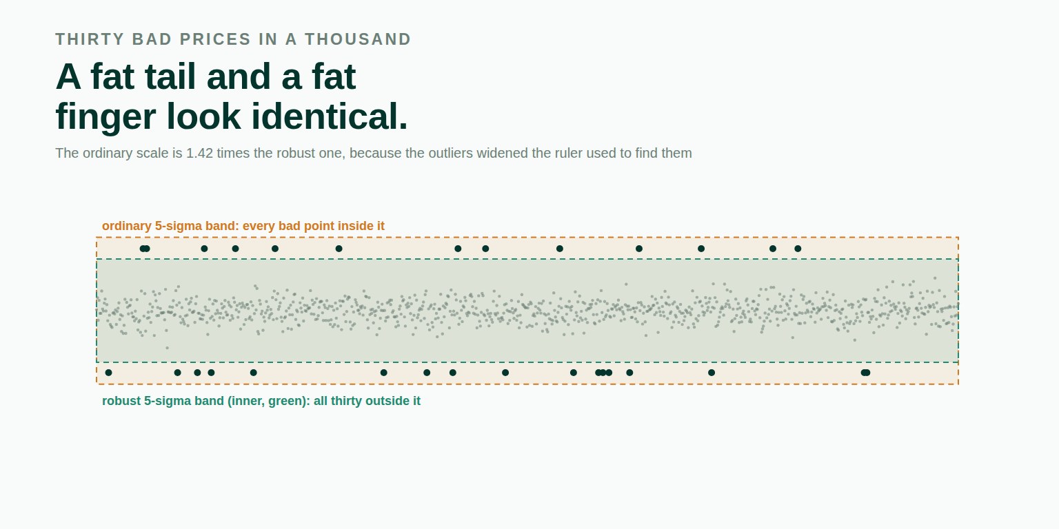
Thirty bad prices hidden in a thousand good ones. A five-sigma z-score finds none of them, because they widened the ruler it measures with. A robust score finds all thirty. And in a second sample, where nothing is an error, six days make the entire return.
A return of five per cent on a quiet day is either the risk you are paid to carry or a price somebody typed with an extra zero. Nothing in the number distinguishes them. The file holds the same value either way.
The usual response is a screen: compute a z-score, flag anything beyond some number of standard deviations, look at it or drop it. That screen has a flaw built into it, and it fails in exactly the situation it exists for.
A z-score divides by a standard deviation computed from the same sample. Every extreme observation inflates that standard deviation. So the more contamination there is, the wider the ruler becomes, and the less extreme each bad point looks when measured against it.
We built a sample to show it. A thousand ordinary daily returns with a standard deviation of one per cent, then thirty of them replaced with values six times that size — the kind of damage a bad feed handler does. Two ways of measuring the spread:
| Centre | Scale | Found at 5 sigma | Found at 4 sigma | |
|---|---|---|---|---|
| Ordinary: mean and standard deviation | −0.000526 | 0.014219 | 0 | 30 |
| Robust: median and scaled MAD | −0.000309 | 0.010001 | 30 | 30 |
The robust scale is the median absolute deviation, multiplied by 1.4826 so that a sigma means the same thing on both rows for clean data. Extremes cannot move a median. That makes it right for detection — and wrong for description, because a scale that ignores the tail by design cannot tell you how fat the tail is. So the library computes both and does not choose between them for you.
The second case is the harder one, because nothing in it is an error. A thousand days of a strategy with a small positive drift and one per cent daily noise, plus eight days on which it made between four and six per cent. That is what a book that is long convexity, or long a handful of event outcomes, can look like.
| Question | Answer |
|---|---|
| Sum of daily returns | 29.58% |
| Largest gains needed to make half of it | 3 days |
| Largest gains needed to make all of it | 6 days |
| The eight largest days by size | 133% of the total |
| Everything else, 992 days | −9.78% |
| Found at 5 sigma: robust / ordinary | 7 / 4 |
Six days out of a thousand make the entire return. The other 992 sum to a loss. Whether this strategy is good is not a statistical question any more; it is a question about six dates, and whether the prices on them were real.
Suppose someone runs a standard cleaning step and winsorises the sample at three sigma. Clipping always lowers measured volatility, which is why people expect it to raise the Sharpe ratio. Here it does the opposite:
| Before | After clipping at 3 sigma | |
|---|---|---|
| Observations touched | — | 10 |
| Daily volatility | 0.009855 | 0.009199 |
| Annualised Sharpe ratio | 0.4764 | 0.2461 |
On a symmetric tail the mean survives and the ratio rises. On a one-sided tail the profit goes with it and the ratio falls. Both are distortions, of opposite sign, from the same routine step, so the library reports the shift without asserting which way it will go.
The measurement functions flag, count and compare. None of them hands back a cleaned series. winsorise exists separately, so that trimming a sample is a deliberate act with a name, rather than a side effect of having looked at the data.
Five sigma, four, three: the threshold is required, and it is a parameter chosen after seeing the data. That makes it exactly the kind of decision a run manifest exists to record, and one of the forks the multiverse analysis counts.
Ordinary and robust scales answer different questions. Returning one without the other would hide the ratio between them, and that ratio — 1.42 in the first example — is the single most useful number for telling whether the extremes are distorting the ruler.
from mdnorm import flag_extremes, clip_effect, concentration

len(flag_extremes(contaminated, sigma=5))               # 0
len(flag_extremes(contaminated, sigma=5, robust=True))  # 30

concentration(strategy, share=Decimal("0.5"))  # 3
concentration(strategy, share=Decimal("1"))    # 6
clip_effect(strategy, sigma=3).sharpe_shift    # 0.5166
$ mdnorm extremes pnl.csv --sigma 5 --robust --tail 10 \
--concentration 0.5 --clip 3Most of this series has been about numbers computed correctly from data that is subtly wrong, or from a choice nobody wrote down. This one is about both at once. Whether a price is a real print is a data question; whether the biggest trade of the day was a trade is too. Whether a five per cent day belongs in the sample is a data question that decides a statistical one, and the statistics cannot answer it back.
Every figure above came from the extremes module of our open-source library, first released in version 1.36.0. Both series are seeded pseudo-random draws, so every figure reproduces exactly on any machine. The first is 1,000 draws of gauss(0, 0.01) from random.Random(3) with 30 positions then replaced by ±0.06, sign drawn from the same generator. The second is 1,000 draws of gauss(0.0001, 0.009) from random.Random(20260920) with 8 positions replaced by uniform(0.04, 0.06); both rounded to ten places. MIT licensed, no runtime dependencies, 1,759 tests, type-checked clean.
pip install market-data-normalizerThe source is on GitHub, the package on PyPI, and the reasoning behind what the library will and will not do is in ROADMAP.md beside the code. Longer write-ups are on our Medium, releases on LinkedIn, and the tooling we run against our own data is in the Console.
The rest of the series is in our blog: how often the book is traded back, a return has to beat something, a maximum drawdown is a maximum, twelve defensible pipelines, one published number and the things we have decided not to build. Public comments on the work are quoted in full with a link to each source on the community page, and the team is on the about page.
We are open to everyone, from independent developers to funds. If something here is wrong, an issue with a concrete input and a statement of what the right answer would be is the most useful form to send it in — a failing test has always been worth more to us than a paragraph that is correct.
Because the ruler is measured with the thing it is measuring. A z-score divides by a standard deviation computed from the same sample, and every extreme observation inflates that standard deviation. In the example in this article thirty bad points in a thousand raised it by 1.42 times, which pushed all thirty from six sigma down to just over four, so a five-sigma screen found none of them. This is called masking.
One that uses the median as the centre and the median absolute deviation, scaled by 1.4826, as the spread. The extremes cannot move either, so the scale stays where the ordinary observations put it. On the same sample the robust score found all thirty at five sigma.
That is a decision with consequences, and they run both ways. Clipping always lowers the measured volatility. If the extremes were symmetric, the mean survives and the ratio rises. If the tail was one-sided, the profit goes with it: in the second example here the annualised Sharpe ratio fell from 0.48 to 0.25 when the sample was clipped at three sigma.
Not from the number. A five per cent day that happened and a five per cent day that was typed wrong are the same value in the file. What the number can tell you is how much rests on it. If six days out of a thousand make the entire return, those six days are the whole question, and they deserve a check against a second source.
No. It flags them, measures what removing them would do, and hands back no trimmed data. A separate function winsorises when that decision has been made deliberately, so trimming a sample is a visible act rather than a side effect of looking at it.
The extremes module of our open-source library, first released in version 1.36.0. Both series are seeded pseudo-random draws stated in the article, so every figure reproduces exactly. MIT licensed, no runtime dependencies, 1,759 tests, type-checked clean.