
HarvestGroup360
© 2026 HarvestGroup360 — a brand operated by AMII LTD.
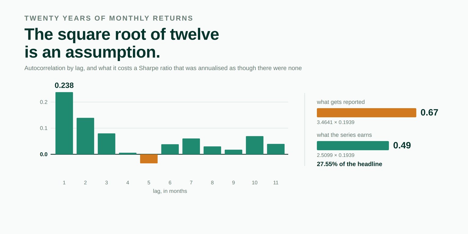
A monthly Sharpe ratio of 0.1939 becomes 0.67 when you multiply it by 3.4641, and 0.49 when you multiply it by the number this particular series entitles you to use. Nothing in the data is wrong. The multiplier is.
There is a number in nearly every performance report that arrived by multiplication rather than by measurement. Somebody computed a Sharpe ratio on monthly returns, multiplied it by the square root of twelve, and wrote down the result. On daily returns the multiplier is the square root of 252.
That step is not questioned, because it does not look like a modelling choice. It looks like converting metres to feet. It is neither: multiplying by the square root of time is a claim that the returns are serially uncorrelated, and it is correct precisely when that claim is true.
Variance adds over time. The variance of a two-period return is the variance of the first period plus the variance of the second, plus twice the covariance between them. If that covariance is zero, the total is simply twice the one-period variance, volatility scales with the square root of the horizon, and a ratio with volatility in its denominator scales with the square root too.
Drop the independence and the covariance term does not vanish. It is added to the multi-period variance, which means the volatility over a year is larger than the calendar suggests, which means the annualised ratio is smaller. The square root of twelve does not know that, so it returns the answer that would have been right for a different series.
The common source of serial correlation in a return stream is not momentum in the asset. It is a mark that was not a trade.
A private position carried at an appraisal value. A corporate bond quoted by a desk rather than crossed on a venue. A model price on an instrument whose last print was Tuesday. In each case the value struck for this period contains part of the previous period's move, because the move had not finished arriving when the value was struck. This is not misconduct and usually not even carelessness — it is what a valuation process does when the market has not yet supplied an answer.
The consequence is mechanical, and it compounds:
| Step | Effect |
|---|---|
| A mark carries part of last period's move | period-to-period variation falls |
| Less variation | measured volatility falls |
| Lower volatility in the denominator | the period Sharpe ratio rises |
| Multiply by √12 | the inflated ratio is scaled, not corrected |
240 monthly returns from a book with partly stale marks. The lag-one autocorrelation is 0.238 — unremarkable, and well inside what a fund with meaningful illiquid exposure reports. The first eleven autocorrelations are in the cover image above; they decay from lag one and one of them is mildly negative.
| Quantity | Value |
|---|---|
| Observations | 240 |
| Sharpe ratio, per month | 0.193901 |
| Autocorrelation, lag 1 | 0.238055 |
| Autocorrelation, lag 2 | 0.139693 |
| Autocorrelation, lag 3 | 0.080109 |
| Naive annualisation factor | 3.464102 |
| Corrected factor | 2.509901 |
| Ratio of the two | 0.724546 |
| Annualised Sharpe ratio | Value | |
|---|---|---|
| As reported | 0.671692 | 3.4641 × 0.1939 |
| As the series supports | 0.486672 | 2.5099 × 0.1939 |
| Difference | 0.185020 | 27.55% of the headline |
Andrew Lo published it in 2002, in The Statistics of Sharpe Ratios. For a horizon of q periods the honest multiplier is:
q / sqrt( q + 2 * sum over k = 1..q-1 of (q - k) * rho_k )
Set every autocorrelation to zero and the sum vanishes, leaving q / √q, which is √q exactly. That is the part worth pausing on. The familiar factor is not the general rule with a correction bolted onto it. It is the special case, and it has been the special case for twenty-four years.
A correction that depends on a single formula is worth cross-checking, so the module reports two other statistics that answer the same question through different arithmetic.
The variance ratio asks directly whether the variance of twelve-month returns is twelve times the variance of one-month returns. Under independence it is one. The long-run variance is the Newey-West figure that belongs under the square root of a standard error once a series is autocorrelated; on an independent series it collapses to the ordinary variance.
| Cross-check | Value | Under independence |
|---|---|---|
| Variance ratio at twelve months | 1.911987 | 1.0 |
| Long-run variance / ordinary variance | 1.904882 | 1.0 |
We report the variance ratio with its bias measured rather than mentioned. It drifts toward one at long horizons, because a twelve-period window fits only n−11 times and those windows share most of their observations. On four thousand draws from a process whose asymptotic ratio at twelve periods is 1.857, our estimator returns about 1.66.
Negative autocorrelation makes the square root of time understate. Bid-ask bounce does it, a mean-reverting spread does it, a market-making book does it. We were tempted to call the gap an overstatement, because that is the interesting case and the one that makes the better headline. It would also have been wrong on roughly half the series it was applied to. So the field is called a difference and a separate flag reports which direction a given series runs.
We had to learn that once already. One release earlier, in the compounding module, we shipped a field whose name asserted a direction the arithmetic does not guarantee, and renamed it afterwards. Better to pay for that lesson once.
Lo's factor wants q−1 autocorrelations. Annualising daily returns wants 251, and nobody has 251 worth trusting — at lag 200 on five years of data the estimate rests on a thousand pairs that mostly overlap. Supplying fewer is the normal case and it treats the rest as zero, which pulls the answer back toward the naive one.
That is the flattering direction on a positively autocorrelated series. So the result carries the lags it used against the lags the horizon wanted, and a truncated answer reads as a lower bound on the correction rather than an estimate of it. On the series above, using only the lag-one autocorrelation gives a factor of 2.890332 against 2.509901 with all eleven — visibly closer to the naive 3.464102, which is exactly the bias being described.
Strong negative autocorrelation at short lags can drive the implied multi-period variance to zero or below. That is not a small scaling factor, it is an absence of one, so the function raises. A constant series raises too, rather than reporting an autocorrelation of zero — zero there would read as evidence of independence instead of absence of data, and those are different statements.
If the book holds anything that does not trade every day, the check takes about five minutes and applies to a figure that has already been published:
from mdnorm import serial_report

rep = serial_report(monthly, periods_per_year=12, max_lag=11)

rep.first_order              # 0.238055
rep.factor.naive             # 3.464102
rep.factor.corrected         # 2.509901
rep.factor.naive_overstates  # True
rep.naive_annualised         # 0.671692
rep.corrected_annualised     # 0.486672
rep.variance_ratio           # 1.911987
$ mdnorm serial monthly.csv --periods 12 --max-lag 11 --show 4 --hac 11Compute the lag-one autocorrelation first. If it is meaningfully above zero, the annualised ratio is overstated and the amount is not a rounding difference. If it is meaningfully below zero, the ratio is understated, which is a different conversation and an equally real one.
It looks like a finance question rather than a normalisation one, and it belongs here for the same reason every other module does: it is a way for a research pipeline to produce a number that is wrong in a direction that flatters, and that class of error does not announce itself.
It is the same shape as an average return nobody received, as a Sharpe ratio that cannot be anything but zero, as counting forty positions as forty bets and as treating overlapping labels as independent observations. Each produces a plausible figure by a defensible route, each errs upward, and none of them raises an exception.
Every figure above came from the serial module of our open-source library, released in version 1.42.0 this morning. The series is a seeded pseudo-random draw — 240 values built as 0.004 + x where x follows x = 0.3 * x + gauss(0, 0.028) from random.Random(20260916), rounded to ten places — so every autocorrelation, both factors and both cross-checks reproduce exactly on any machine. MIT licensed, no runtime dependencies, 1,648 tests, type-checked clean. The method is Lo (2002), The Statistics of Sharpe Ratios, Financial Analysts Journal 58(4).
pip install market-data-normalizerThe source is on GitHub, the package on PyPI, and the reasoning behind what the library will and will not do is in ROADMAP.md beside the code. Longer write-ups are on our Medium, releases on LinkedIn, and the tooling we run against our own data is in the Console.
The rest of the series is in our blog: the average return nobody received, the Sharpe ratio of a residual, why forty positions is not forty bets, twelve defensible pipelines and one published number and the things we have decided not to build. Public comments on the work are quoted in full with a link to each source on the community page, and the team is on the about page.
We are open to everyone, from independent developers to funds. If something here is wrong, an issue with a concrete input and a statement of what the right answer would be is the most useful form to send it in — a failing test has always been worth more to us than a paragraph that is correct.
Because multiplying by the square root of the calendar is only correct when each period's return is independent of the one before it. The square root comes from variance adding linearly over time, and variance adds linearly only under independence. If the returns are serially correlated the multi-period variance is larger or smaller than the calendar implies, and the familiar factor is simply the wrong number.
Most often, a mark that is not a trade. An appraisal valuation, a dealer quote on a bond that did not change hands, a model price on an instrument whose last print was days ago — each carries part of the previous period's move into the current one, because the move had not finished arriving when the mark was struck. Genuine momentum or mean reversion in the asset does it too, but stale valuation is the common case and the one that flatters.
On the series in this article, a lag-one autocorrelation of 0.238 turns a naive annualised Sharpe of 0.671692 into 0.486672 — 27.55 per cent of the headline figure. That autocorrelation is unremarkable; funds with meaningful illiquid exposure regularly report higher.
No. Negative autocorrelation — bid-ask bounce, a mean-reverting spread, a market-making book — makes the square root of time understate rather than overstate. That is why our report names the quantity a difference rather than an overstatement and carries a separate flag for which direction a given series runs. A name that asserted a direction would be wrong about half the series it was applied to.
Lo's factor needs an autocorrelation for every lag from one to q minus one. Annualising daily returns needs 251 of them, and past the first handful they rest on too few pairs to be worth anything. Supplying fewer is normal and treats the rest as zero, which pulls the result back toward the naive answer. On a positively autocorrelated series that is the flattering direction, so a truncated result is a lower bound on the correction rather than an estimate of it, and the report says how many lags it used against how many the horizon wanted.
Yes, and it is worth doing as a cross-check. The variance ratio asks whether the variance of q-period returns is q times the variance of one-period returns, and the Newey-West long-run variance asks the same question in the form that belongs under a standard error. On the series here they come out at 1.911987 and 1.904882 times the ordinary variance, which agree with each other and with the scaling factor.
The serial module of our open-source library, released in version 1.42.0. The series is a seeded pseudo-random draw stated in the article, so every autocorrelation and both factors reproduce exactly on any machine. MIT licensed, no runtime dependencies, 1,648 tests, type-checked clean.