
HarvestGroup360
© 2026 HarvestGroup360 — a brand operated by AMII LTD.
Subtract the factors, measure what is left, report the ratio. The procedure is right, the order is right, and the number it produces is zero for every strategy ever written — because of how least squares works, not because of how the strategy performed.
A claim of alpha is a claim about a remainder. The strategy made money; some of that is market exposure anybody can buy for a few basis points, and the interesting question is what survives once the purchasable part is taken out. Regress the return stream on the factors, keep the residuals, and measure those.
This is the correct procedure. It also contains a trap that is easy to walk into and produces a result that looks like an answer, which is the combination worth writing about.
Ordinary least squares with an intercept forces the residuals to sum to zero. That is not an approximation or a tendency; it is what fitting an intercept does. The mean of the residual series is therefore zero to the last digit the arithmetic carries.
A Sharpe ratio is a mean divided by a standard deviation. With a numerator that is exactly zero, the ratio is exactly zero — for a brilliant strategy, for a worthless one, for a series of random numbers. In the worked case below it comes out as 4.6×10−36, which is zero plus forty digits of decimal round-off.
This was our own mistake. An early version of this module recommended exactly this in a docstring: fit the regression, take the residuals, hand them to the Sharpe function. The API now has two separate functions, and the reason is in the changelog.
Add the intercept back. The residuals answer how far was each day from the fitted line; the alpha stream answers what did each day contribute that the factors do not explain. They differ by exactly the alpha at every observation, and only one of them has a mean worth dividing by.
| Series | Mean | Useful for |
|---|---|---|
residuals() | zero by construction | diagnostics — autocorrelation, heteroskedasticity, outlier days |
alpha_stream() | the alpha | any statistic that reads the level — Sharpe, drawdown, hit rate |
The alpha stream is also the series to feed back into the rest of the library. A window sweep over the alpha stream asks whether the edge survives when the sample is trimmed, which is a sharper question than asking it of the raw returns — because the raw returns contain a market exposure that trims well for reasons having nothing to do with the strategy.
1,260 daily returns from a strategy built on a market factor, a value factor and a momentum factor, with a small planted edge and its own noise. The regression recovers the structure:
| Factor | Loading | Standard error | Contribution to mean return |
|---|---|---|---|
| market | 1.1382 | 0.0083 | +0.00043106 |
| momentum | 0.4816 | 0.0139 | +0.00005603 |
| value | −0.2155 | 0.0164 | −0.00004935 |
| alpha | — | 0.0000850 | +0.00009960 |
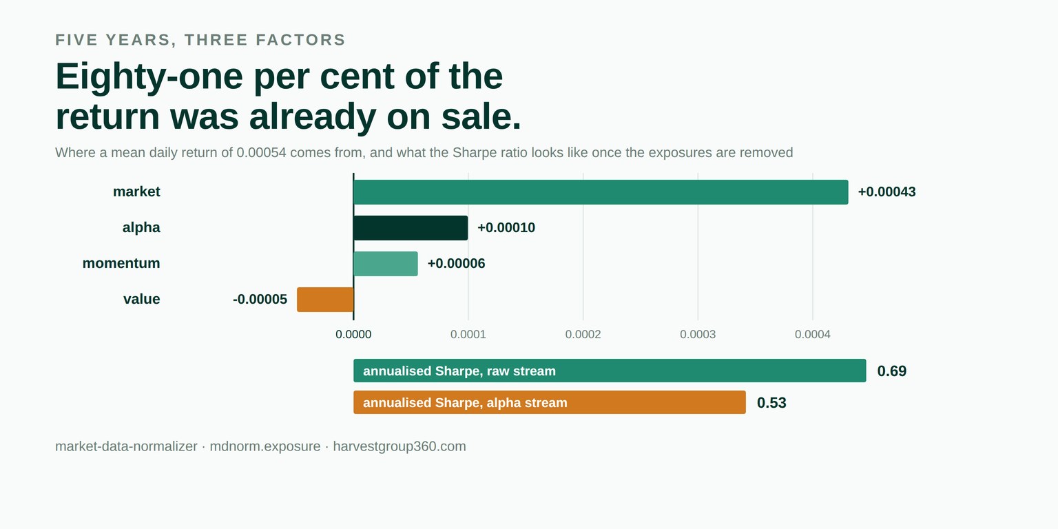
The market loading is 1.138 and the market did well over the sample, so the market alone carries 0.00043 of the 0.00054 the strategy earned. That is 80 per cent of the return from an exposure that costs a few basis points to hold. Alpha accounts for 18.5 per cent; the two remaining factors roughly cancel.
Note which factor dominates. Momentum has a loading of 0.48, more than twice the size of the value loading, and it contributes barely more than value takes away — because contribution is the loading multiplied by what the factor actually did, and a large exposure to a factor that went nowhere earns nothing. Ranking by coefficient size would have put the wrong name at the top.
| Measure | Raw return stream | Alpha stream |
|---|---|---|
| Sharpe ratio (per period) | 0.0433 | 0.0331 |
| Annualised at 252 | 0.69 | 0.53 |
| Residual stream, for comparison | — | 0.0000 — zero by construction |
A drop from 0.69 to 0.53 is not catastrophic, and we would rather show a case like this than construct one where the edge vanishes. Most of the Sharpe survives here because the noise term is large relative to the factor exposure, so removing the exposure removes return and risk together. A strategy that was mostly beta with a thin overlay would lose far more, and the arithmetic is the same either way.
The intercept is 0.00009960 with a standard error of 0.0000850, giving a t statistic of 1.172. Over 1,260 observations that does not clear any conventional bar.
It is worth being precise about what that does and does not mean. It does not mean the alpha is zero — there is a planted edge in this series and the estimate recovers it to within a standard error. It means five years of daily data cannot distinguish this intercept from zero. The strategy might be fine; the evidence is thin. Those are different sentences and a report that only carried the point estimate would let them blur.
from mdnorm.exposure import (factor_regression, alpha_stream,
                             residuals, dominant_factor)

rep = factor_regression(strategy, {"market": mkt, "value": val,
                                  "momentum": mom})

rep.r_squared            # 0.9413
rep.alpha                # 0.00009960
rep.alpha_standard_error # 0.00008497
rep.alpha_t_stat         # 1.1722
rep.alpha_share          # 0.1854   <- 18.5% of the mean return
rep.explained_share      # 0.8146
rep.crowded              # False

dominant_factor(rep).name        # 'market', ranked by contribution

sharpe_ratio(alpha_stream(strategy, factors))   # 0.0331
sharpe_ratio(residuals(strategy, factors))      # 0.0000, always
The matrix inversion runs in exact decimal arithmetic at fifty digits of precision, and a design that is singular raises rather than returning one of the infinitely many possible answers. The error names the offending column: two identical factors, a factor that is the sum of two others, or a constant column that is the intercept under another name. “Singular matrix” tells a caller nothing they can act on; “the design is singular at momentum” tells them where to look.
The report also flags a crowded regression — too many factors for the observations available — without refusing to run it, because how much room a fit needs is a judgement about the question rather than a property the library can settle.
Alpha is defined relative to a factor set. Add a factor and the intercept usually shrinks; the strategy has not changed. A result that says “alpha of 0.0001 after three factors” is a complete sentence and “alpha of 0.0001” is not. Which factors belong in the regression is exactly the kind of decision that belongs in a specification grid.
Strategies with options, stops or dynamic leverage have returns that are not linear in the factors, and a linear regression will report an intercept for them that is partly a misspecification rather than an edge. Nothing in the residual diagnostics will necessarily make that obvious. The module does not detect nonlinearity and does not claim to.
A strategy whose market exposure was 0.4 in the first two years and 1.8 in the last three reports a single loading somewhere in between, which describes no period. The regression has no time dimension. Running it over rolling windows is the check, and it is the caller's to run.
Every figure above came from the exposure module of our open-source library, released in version 1.40.0, run against the Sharpe implementation in the same package. The panel is a seeded pseudo-random draw — 1,260 observations from random.Random(20260914), three factors and a strategy built with loadings of 1.14, −0.22 and 0.46 on them plus an alpha of 0.00007 and gauss(0, 0.0031) of noise — so every loading, the intercept and both Sharpe ratios reproduce exactly on any machine, including the t statistic that fails to clear a bar. MIT licensed, no runtime dependencies, 1,608 tests, type-checked clean.
pip install market-data-normalizerThe source is on GitHub, the package on PyPI, and the reasoning behind what the library will and will not do is in ROADMAP.md beside the code. Longer write-ups are on our Medium, releases on LinkedIn, and the tooling we run against our own data is in the Console.
The rest of the series is in our blog: why forty positions is not forty bets, twelve defensible pipelines and one published number, the start date somebody chose, the file that did not change while the answer did and the things we have decided not to build. Public comments on the work are quoted in full with a link to each source on the community page, and the team is on the about page.
We are open to everyone, from independent developers to funds. If something here is wrong, an issue with a concrete input and a statement of what the right answer would be is the most useful form to send it in — a failing test has always been worth more to us than a paragraph that is correct.
Because an intercept absorbs the mean exactly. Ordinary least squares with a constant term forces the residuals to sum to zero, so their mean is zero to machine precision, so any ratio with that mean in the numerator is zero. It is zero for a brilliant strategy and for a worthless one, which makes it a property of the arithmetic rather than a statement about the return stream.
The residual series with the intercept added back to every observation. Its mean is the alpha, its variance is the residual variance, and a Sharpe ratio on it means what a reader would expect the phrase to mean: reward per unit of risk on the part of the return the factors do not explain. The two series differ by exactly the alpha at every point.
No. It means most of the variance is explained by the factors supplied, which is a statement about those factors as much as about the strategy. A strategy can have a high R-squared and a real intercept. What a high R-squared does rule out is describing the return stream as independent of the market when it demonstrably is not.
Usually not. A loading of 9 on a factor that went nowhere contributes nothing to the return, and a loading of 0.2 on a factor that moved a lot contributes a great deal. The library ranks factors by contribution — the loading multiplied by the factor's own mean — rather than by the size of the coefficient, because the coefficient alone answers a different question.
The regression is refused and the offending column is named. A singular design has no unique solution, and a library that quietly returned one of the infinitely many possible answers would be handing back a number with no meaning. The error names the factor rather than saying 'singular matrix', because the name is the part a caller can act on.
No, and the distinction is worth keeping. An insignificant alpha means the data cannot distinguish it from zero over the sample available. That is a statement about the evidence, not about the strategy. The report carries the standard error and the t statistic alongside the estimate precisely so the two do not get confused.
The exposure module of our open-source library, released in version 1.40.0. The panel is a seeded pseudo-random draw stated in the article, so the loadings, the intercept and both Sharpe ratios reproduce exactly on any machine. MIT licensed, no runtime dependencies, 1,608 tests, type-checked clean.