
HarvestGroup360
© 2026 HarvestGroup360 — a brand operated by AMII LTD.
Everybody removes the shape of the trading day before measuring anything inside it. Very few people check whether the shape they removed it with had happened yet.
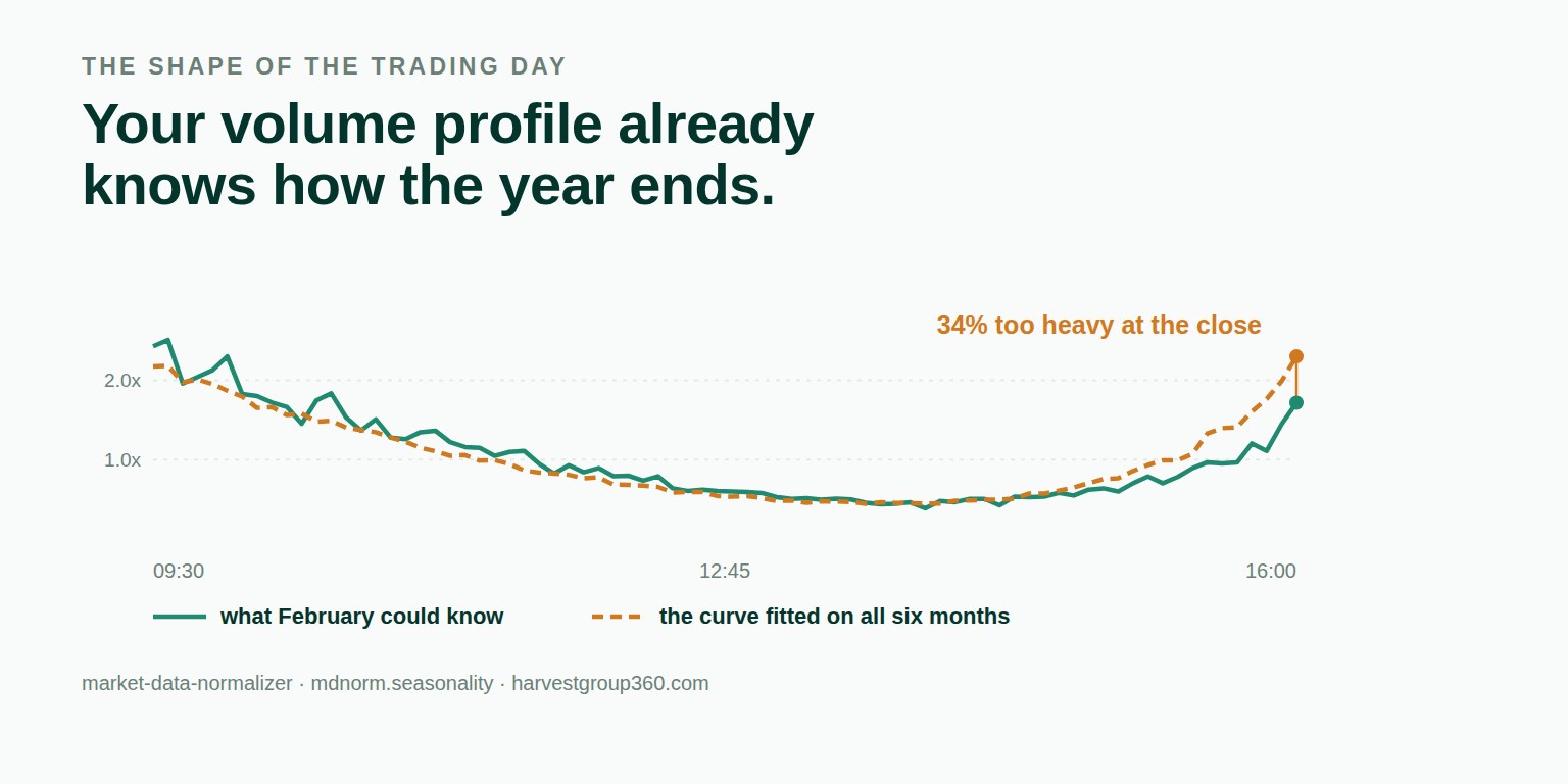
Activity inside a session is not flat. On most equity venues it is a U: heavy in the first minutes, thin around midday, heavy again into the close. The same curve shows up in spreads, in trade counts and in realised volatility. Any intraday statistic computed without accounting for it is mostly measuring the clock.
So the curve gets divided out, and the recipe is old and universal: average each five-minute slot across the sample, express it as a multiple of the day, divide every observation by its slot's multiple. Two lines of code, and after them a volume reading means something comparable at 09:31 and at 13:00.
Most look-ahead has an obvious shape. Reading a close before the session ended, buying a stock the index added next month, joining a quarterly figure at the quarter it describes rather than the day it was published — each of those is a value appearing before its own timestamp, and once somebody points at it the argument is over.
A seasonality profile is not a value. It is a parameter, and parameters do not feel like data. Nobody writing volume / profile[slot] thinks of it as reading the future, because the thing being read is a shape rather than a number, and the shape feels like a property of the venue: a fact about how markets work, not an observation with a date on it.
It has a date on it. The curve is an estimate from a specific set of days, and every day in that set is a day somebody had to live through first.
How much this matters depends entirely on how stable the curve is. If a venue's day looked the same in January as in June, the two approaches agree to the last digit and there is nothing here to fix. That case is real and it is common, and we would rather say so than sell a problem nobody has.
The case that is also real: a closing auction that grows. Below is six months of five-minute volume, 120 sessions and 9,360 observations, simulated with a closing weight that rises steadily across the sample and lognormal noise on every point. Synthetic on purpose — we would rather publish a generator you can re-run than a client capture you cannot.
| Five minutes ending | Multiple of the day |
|---|---|
| 09:35 — the opening bucket | 2.17× |
| 10:35 | 1.49× |
| 12:50 | 0.53× |
| 13:35 — the quietest bucket | 0.44× |
| 15:50 | 1.76× |
| 16:00 — the closing bucket | 2.30× |
An ordinary U, and a perfectly good description of what that venue's day looks like over those six months. Now the same curve fitted the other way — one profile per session, built only from the sessions before it — and compared with the full-sample one, factor by factor:
| Comparison across 7,800 adjustable observations | Value |
|---|---|
| Factors that differ by more than 1% | 6,453 (82.73%) |
| Median disagreement | 4.03% |
| Largest disagreement | 59.04% |
The disagreement is not spread evenly, and where it concentrates is the whole story. In early February the full-sample profile divides the closing five minutes by 2.30×. The curve available at that moment said 1.72×. That is 34% too heavy, and all of it comes from a closing auction that had not grown yet.
Divide by a factor that is a third too large and the adjusted value comes out a quarter too small. Do that only in the early part of the sample, where the fitted curve is furthest from what was known, and the adjusted series acquires a slope that is not in the data:
| Closing bucket, adjusted | Full-sample ÷ point-in-time |
|---|---|
| First month after the warm-up | 0.754 |
| Final month | 0.981 |
Read across that table and the size of it lands: the adjustment alone puts roughly 30% of upward drift into the adjusted closing series over six months. Not the market — the normalisation. Any study of whether closing activity is trending has that baked into it before it starts, pointing the same way as the thing it is looking for.
Having measured the distortion, the obvious next question is what it does downstream. We ran the plainest thing we could think of: a rolling three-sigma flag over both adjusted series, on identical data, counting how many observations each one calls an outlier.
Seventy-four for the point-in-time series. Seventy-two for the full-sample one. Two.
That is not the result we expected and we are reporting it because it is the result. It also explains the whole problem better than a dramatic number would have. The distortion here is not spiky — it does not manufacture events that get flagged and investigated. It is a smooth, one-directional shift in level that moves slowly across the sample. It passes every sanity check anybody runs, because sanity checks look for things that stick out, and this does the opposite: it makes the early sample slightly quieter and the late sample slightly noisier, forever, in a way that looks like a finding.
The fix is not clever. Fit one profile per session from the sessions before it, and use that. Everything interesting is in what the implementation refuses to do.
Both fits are in the library. The full-sample one is genuinely the better estimate of how a venue's day is shaped — it uses every observation — and genuinely the wrong input to anything that trades. Those are different jobs, and a library that shipped only the safe one would be making a judgement it cannot make on your behalf. It also would not be able to measure the gap, and a difference nobody can compute is a difference nobody checks.
A profile built from three sessions is one day's noise wearing a curve's clothes, and dividing by it invents outliers rather than removing them. So the first sessions produce no adjusted output at all. A gap in the series is a visible cost; a number nobody can defend is an invisible one, and this library takes the visible one every time — the same rule that stops a rolling window emitting anything before it is full.
The tempting fallback is to fill a sparse slot with the overall mean, which makes the adjusted series look well behaved in precisely the places where nothing is known about it. A bucket below the evidence threshold comes back empty, and a point with no factor leaves the output, because a point silently divided by one is a point claiming to have been adjusted.
Five minutes over a 6½-hour session is 78 buckets; the same five minutes on a venue that never closes is 288. Finer buckets describe the curve better and put less evidence in each, and where that trade sits is a property of your data. The library asks, for the same reason it ships no default number of sessions in a year and no default tick size.
Buckets are measured as an offset from the open, so on a half-day the closing surge lands in a slot that is the middle of the afternoon on every other day. That spoils the profile in two places at once. Given a trading calendar the early closes are excluded and the count is reported; without one every day is treated as full length, which is a claim, so the number of sessions actually used is always printed.
$ mdnorm seasonality volume.csv --session 09:30-16:00 \
      --tz America/New_York --bucket 5m --min-sessions 20
sessions used        120
buckets              78 of 5m
buckets with no data 0
heaviest bucket      +6h25m into the session (2.30x)
lightest bucket      +4h into the session (0.44x)
comparable samples   7800 of 9360
factor differs by    >0.01: 6453 (82.73%)
median gap           4.03%
largest gap 59.04%Every parameter estimated over a whole sample and applied back to the start of it has this property. A volatility scaling factor. A winsorising threshold. A PCA basis. A set of feature means and standard deviations fitted before the train-test split. None of them look like reading the future, because none of them are values — and all of them carry a date regardless.
The test we use is short. Could this number have been computed on the morning it is applied? If not, it is an input from the future, whatever it is called. The answer is usually no, and usually the fix costs a warm-up period and a slightly uglier chart.
The measurements above come from the seasonality module of our open-source library, released in version 1.28.0. It is MIT licensed, has no runtime dependencies, ships 1,109 tests and passes a type checker clean.
pip install market-data-normalizerThe test suite is the part we would point at first, and one test in particular: it gives a single session a wildly different shape and asserts that the profile handed to that session is identical to a profile of the days before it. That property is the entire module, and it is checked rather than claimed.
The source is on GitHub and the package on PyPI. What the library will and will not do, with the reasoning next to each entry, is in ROADMAP.md and BENCHMARKS.md. Longer write-ups are on our Medium, releases and the discussion around them on LinkedIn, and the tooling we run against our own market data is in the Console.
The rest of the series is in our blog: the delay between a venue stamp and an arrival, the things we have decided not to build, telling real prints from arithmetic, a trading year that was not 252 sessions, a universe chosen with hindsight and a value read before it was published. Comments on the work, quoted in full with a link to each source, are on the community page, and the team is on the about page. Newer in the same series: the average return nobody received.
If something here is wrong, an issue with a concrete input and a statement of the right answer is the most useful form to send it in. We are open to everyone, from independent developers to funds, and a failing test has always been worth more to us than a paragraph that is correct.
The average shape of activity within a trading session, measured in slots of a fixed width — five minutes, say — across many days. On most equity venues it is a U: heavy in the first minutes, thin around midday, heavy again into the close. The same shape appears in spreads, in trade counts and in realised volatility, which is why almost every intraday statistic has to account for it before it means anything.
Because without it the statistic mostly measures the clock. A volume reading that is twice the daily average is unremarkable at 09:31 and extraordinary at 13:00, and an anomaly detector that does not know which one it is looking at will fire every morning and miss every quiet-hour surge.
In how the profile is fitted. The standard recipe estimates one curve over the entire sample and applies it to every day in that sample, including the first. That curve contains days that had not happened yet, so an early observation is being judged against a shape it could not have known. Nothing about the arithmetic is wrong; the curve is simply not information that existed at the time.
It depends entirely on how much the shape moves over the sample. Where it is stable, the two approaches agree to the last digit and there is nothing to fix. In the six-month example in this article, where the closing auction grows steadily, the full-sample profile makes the closing bucket 34% heavier than the curve available in February, and the adjusted closing series picks up roughly 30% of upward drift from the method alone.
A profile recomputed for each session using only the sessions before it. The curve applied on 3 March contains January and February and nothing after. It is noisier than the full-sample fit, particularly at the start, and that noise is the honest size of what was known.
No, and that is worth being precise about. If the question is what a venue's trading day looks like, the full-sample fit is the better estimate, because it uses every observation. It is only wrong as an input to something that trades, where the requirement is not accuracy but availability. Both belong in a toolkit, and the reason to ship both is that a difference nobody can compute is a difference nobody checks.
More than you would like, and the honest answer is that the library will not guess for you. A profile built from three sessions is one day's noise wearing a curve's clothes, and dividing by it manufactures outliers rather than removing them. Set a minimum, accept that the sessions before it produce no adjusted output at all, and prefer a gap in the series to a number nobody can defend.
It should report nothing. The tempting alternative is to fill it with the overall average, which makes the adjusted series look well behaved in exactly the places where nothing is known about it. A point with no factor is better dropped than passed through unchanged, because a point silently divided by one is a point claiming to have been adjusted.
Yes, and it is easy to miss. Buckets are measured as an offset from the open, so on an early-close day the closing surge lands in a slot that is the middle of the afternoon on every other day. That contaminates the profile in two places at once. Given a trading calendar, short sessions should be left out of the fit and the count of exclusions reported.